About the Author
The author, who has focused on pricing and risk management of stable value products at the Reinsurance Group of America, is also a Fellow of the Society of Actuaries, a Chartered Financial Analyst®, and a Financial Risk Manager.

Summary
As retirement begins, retirees are no longer making regular contributions to their retirement savings, but instead making regular withdrawals. This shift from accumulation to decumulation exposes retirees to “sequence-of-returns risk.” Sequence-of-returns risk is the risk that a sharp decline in the market value of risky assets will occur early in retirement, and that retirees’ regular withdrawals from the portfolio will lock in a meaningful portion of these losses by selling the risky assets at depressed prices, so that even if subsequent returns are favorable, the portfolio will be rapidly depleted.
One way to protect against sequence-of-returns risk and to improve the probability that a portfolio lasts through retirement is to begin retirement with a more conservative allocation and then allow portfolio risk to increase later in retirement (as previously demonstrated by Wade Pfau and Michael Kitces [1]). A simple way of implementing this strategy is to fund several years of withdrawals in advance by placing that money in a low-risk investment and investing the remaining assets more aggressively. Withdrawals are then taken from the low-risk portion of the portfolio, while leaving the riskier portion untouched for years. This type of investment strategy, where investment in low-risk assets peaks near retirement age, has also been referred to as a “bond tent” (the percentage allocation to low-risk assets increases before retirement, peaks at retirement, and then declines, making a triangular pattern that looks like a tent).
Stable value funds, commonly found in 401(k) plans and other retirement plans, are an attractive option for the low-risk portion of the portfolio, as they combine the higher returns and interest rate responsiveness of short-term bond funds with the principal protection of money market funds [2]. Principal protection is desirable when funding steady withdrawals in retirement, as this allows the retiree to avoid the risk of selling investments at depressed market values to fund living expenses. Interest rate responsiveness allows the fund to benefit more quickly from a rising rate environment, which may prove helpful if inflation picks up during retirement. Intermediate-term and long-term bond funds are not principal-protected, and the higher-yielding longer-maturity bonds they hold leave them exposed to the risk of significant losses if interest rates rise. To determine an appropriate allocation to stable value as retirement begins, “backtesting” can be used. Backtesting uses a model to estimate how different allocations would have performed during various historical time periods. By modeling the performance of different allocations during 30-year retirements that start between 1910 and 1990, the allocations that have best supported different levels of withdrawals during retirement can be determined. Withdrawals are summarized by the retiree’s anticipated withdrawal rate, which is the amount needed from the portfolio expressed as a percentage of the initial portfolio value. These withdrawal amounts are adjusted for inflation as retirement progresses to maintain the retiree’s standard of living. The withdrawal rate is calculated from only the initial withdrawal – subsequent withdrawal amounts are the same dollar amount every year, after adjusting for inflation. The retiree’s portfolio is assumed to consist of a mix of stable value and a passive equity fund that tracks the S&P 500 index. The retiree’s initial allocation to stable value is intended to cover a certain number of years of withdrawals before the retiree starts to draw down on the riskier portion of the portfolio that was invested in equities. This backtesting suggests the following allocations will maximize the probability that a retirement portfolio provides at least 30 years of inflation-adjusted withdrawals:
Note that these allocations to stable value are as of the date that retirement begins. During retirement, the stable value allocation will tend to decrease as it is spent down, and the equity allocation will tend to increase since it can grow untouched until the stable value allocation is depleted.
For the lowest withdrawal rates (4.0% or less), there is substantial leeway to adjust the initial portfolio composition, as many portfolio allocations will allow the portfolio to support 30 years of withdrawals. For the highest withdrawal rates (over 7.0%), placing almost the entire portfolio in riskier, higher-yielding assets may offer the best chance of having the portfolio support 30 years of withdrawals.
This strategy may need to be adjusted to account for the particular circumstances that a retiree faces. In particular, modifications may be needed if the portfolio includes risky assets other than domestic equities, if retirement is expected to last longer than or shorter than 30 years, or if the retiree has a strong desire to leave the largest possible bequest. In addition, the analysis that was used to develop this strategy was based solely on historical data, so it cannot capture changes in our economy or financial markets that may occur.
Detailed Analysis
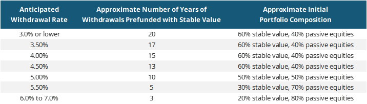
By starting retirement with a significant allocation to stable value, the retiree’s portfolio is protected at the time when it is most susceptible to a prolonged market downturn. To estimate the optimal balance between the protection provided by the stable value allocation and the opportunity for higher returns provided by the allocation to riskier assets, backtesting can be used to look at how different allocations would have performed in the past. Retirees with different withdrawal rates have part of their portfolio invested in a hypothetical stable value fund, with the remainder invested in a passive equity fund that tracks the S&P 500 index. In order to capture a broader variety of market conditions, this backtesting covers the period from 1910 through 2020. Because neither stable value products nor the S&P 500 index existed at the beginning of this study period, historical data has been used to reconstruct how they would have behaved. In particular, the hypothetical stable value fund used here credits interest based on a 5-year moving average of 5-year Treasury rates (replicating the average book yield from buying 5-year bonds and holding them to maturity), plus an additional 0.50% (intended to capture the portfolio’s credit spread). The retiree will fund withdrawals from the stable value allocation until it is depleted, and then draw on the equity portion of the portfolio. Withdrawals are adjusted for inflation to maintain the retiree’s standard of living. For a specific example of how this strategy works, consider a retiree with a $1 million portfolio seeking to withdraw an inflation-adjusted $45,000 annually. The retiree begins retirement in 1929, immediately before the Great Depression. The retiree’s initial allocation to stable value is 67.5%, which funds 15 years of anticipated withdrawals, with the balance of the portfolio invested in equities. Inflation-adjusted withdrawals are taken from the stable value allocation until it is exhausted. With this approach, the equity portion of the portfolio is left untouched for many years and is able to participate in the eventual market recovery:
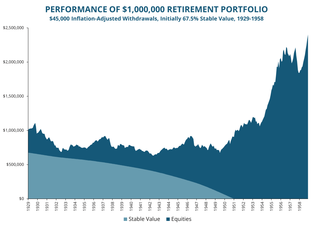
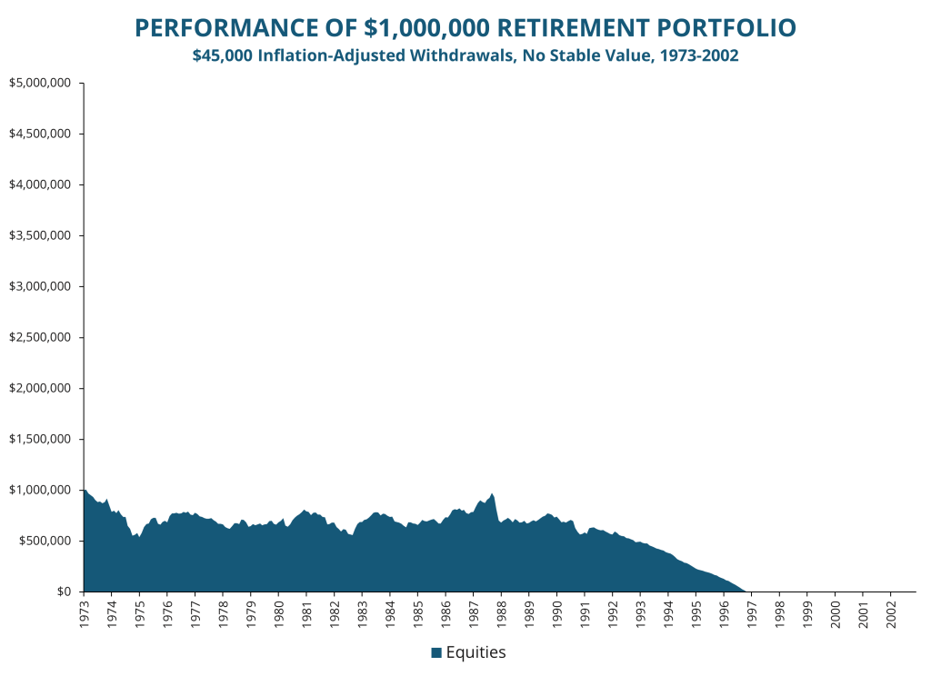
If, however, the retiree invests only in equities, the combination of a market crash and steady withdrawals means that the portfolio is depleted too quickly to participate in the eventual recovery:
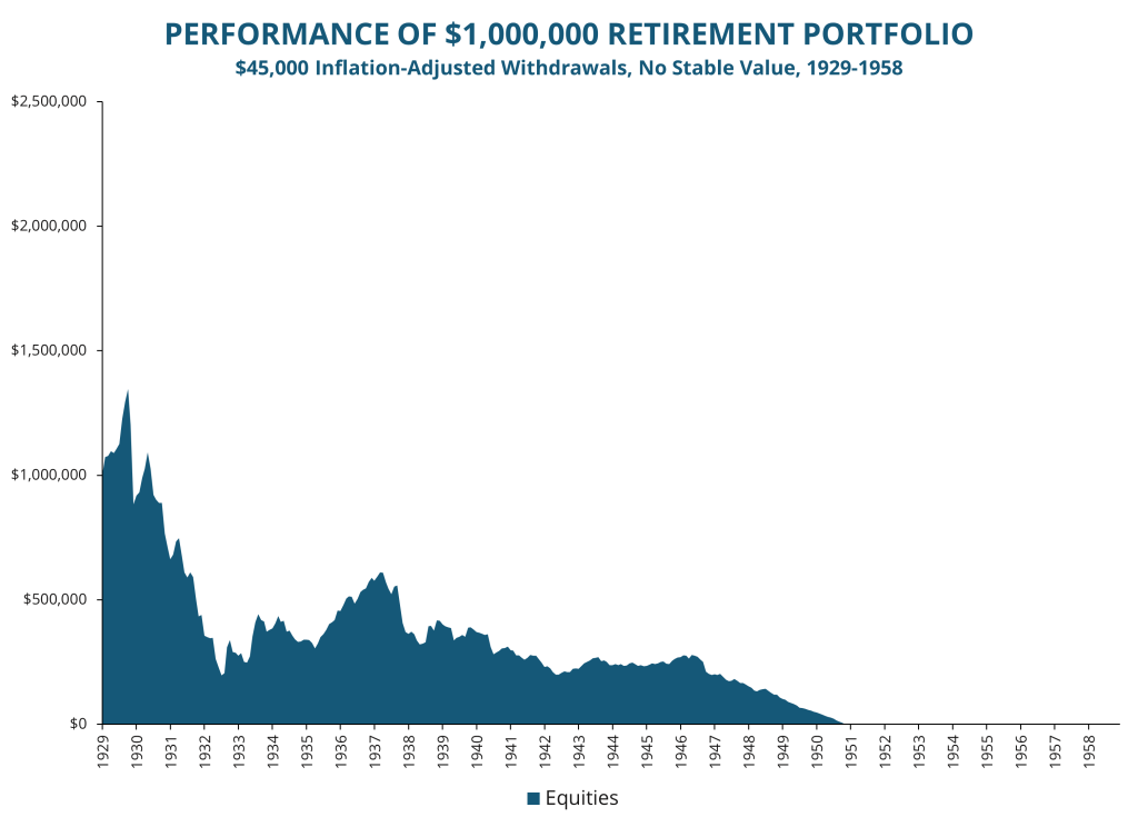
In a similar vein, consider another retiree who begins retirement in 1972, immediately before a period of poor equity returns and high inflation. By prefunding the first 15 years of anticipated withdrawals with a 67.5% initial allocation to stable value, the retiree’s portfolio supports the desired withdrawals throughout this challenging period:
Modeling the portfolio with a 4.5% withdrawal rate with varying initial allocations to stable value reveals that a portfolio starting with a 65%-70% allocation to stable value (which corresponds to 15 years of 4.5% withdrawals in the below chart) can survive 30 years with 98% probability.
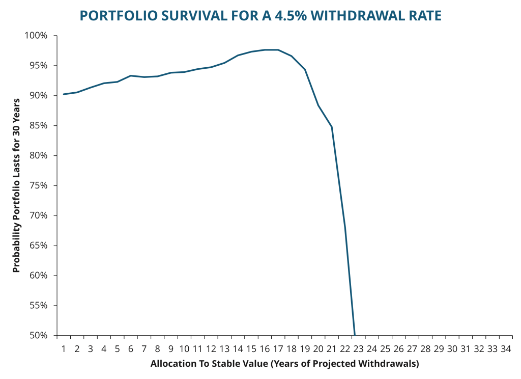
As the initial stable value allocation increases beyond 70%, the probability that the portfolio survives 30 years of withdrawals begins to decline, with a sharper drop off after the stable value allocation increases past 85% (or about 19 years of projected withdrawals). The stable value allocation should be large enough so that the retiree doesn’t have to touch the equity allocation for some time, so that it can grow unimpeded, but the equity allocation also needs to be large enough so that it can grow to cover the remaining years of retirement.
At different withdrawal rates, there can be a different optimal balance between protection from market movements in the early years of retirement and portfolio growth to support the later years of retirement. When a retiree has a moderate withdrawal rate, like the 4.5% used for the prior example, there’s a narrow range of allocations to stable value that produce the highest probability that the portfolio will last 30 years. However, if a retiree has a low withdrawal rate, a wide range of portfolio strategies are likely to resist depletion over 30 years. At the other extreme, if a retiree has an extremely high withdrawal rate, no portfolio strategy is likely to support the retiree for 30 years. High withdrawal rates tend to produce low survival rates, even with optimal investment allocations, since success depends on being in an era with consistently high investment returns. This can be seen by looking at how portfolios for retirees with different withdrawal rates (abbreviated “W/D,” and ranging from 3% to 7%) perform in all possible 30-year scenarios starting between January 1910 and January 1991:
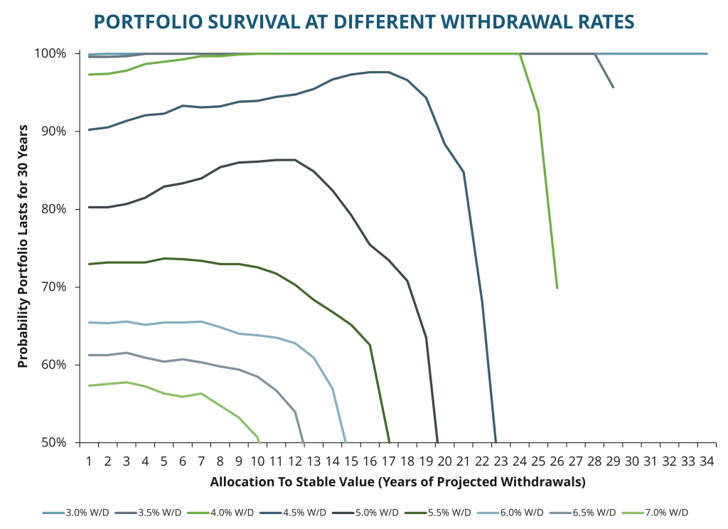
The lower withdrawal rates (3.0% to 4.0%) each have multiple allocations that produce a 100% survival rate during the time periods used in backtesting. This is why their survival rate graphs have flat, horizontal sections corresponding to 100% survival above. For the highest withdrawal rates (5.5% and above), survival rates are lower, and the optimal portfolio tends to involve a much smaller allocation to stable value.
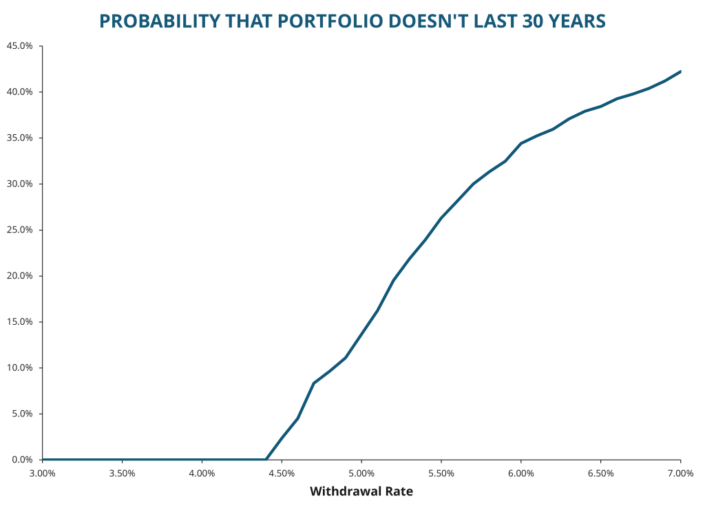
In view of the optimal allocation for each withdrawal rate, the probability that the portfolio fails to provide 30 years of withdrawals begins to increase steadily as withdrawal rates increase:
The range defined by the highest and lowest levels of prefunding that allow the portfolio to survive 30 years of withdrawals with a probability no more than one percent lower than the optimum can be used to see what portfolios are most likely to support 30 years of retirement. For very low withdrawal rates there is a broad range of allocations that is likely to provide 30 years of withdrawals. However, as withdrawal rates increase, there is less room for error, and the range of prefunding that produces a near-optimal outcome shrinks:
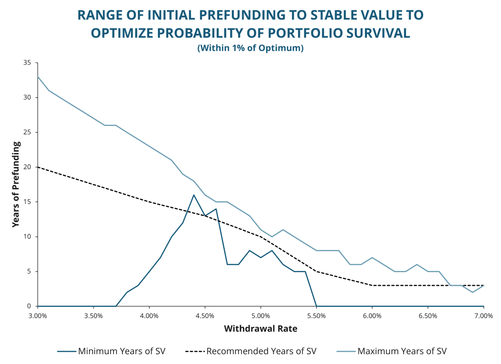
The dashed line in this graph corresponds to the recommendations given in the table in the strategy overview at the beginning of this paper.
The degree of prefunding can also be expressed as the initial percentage allocation to stable value in the portfolio, and the range of near-optimal initial allocations exhibits similar behavior:
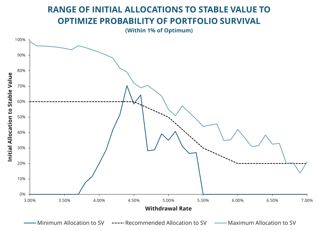
As in the preceding graph, the dashed line corresponds to the recommendations given in the table in the strategy overview at the beginning of this paper.
The recommendations given at the beginning of the paper are based on these backtesting results. As can be seen above, there is considerable leeway to adjust the stable value allocation upward or downward if the anticipated withdrawal rate for the retiree is under 4%. Similarly, as withdrawal rates rise well above 6%, the retiree can consider lowering the initial allocation to stable value below the recommended level of approximately 20%.
Strategy Adjustments
In this analysis, the risky portion of the portfolio is assumed to be invested solely in the S&P 500. A different mix of riskier assets that includes high-yield bonds, long-term bonds, small-cap equities, international equities, and other asset classes may have a different expected return and risk profile. Lowering the risk of this portion of the portfolio would suggest a smaller allocation to stable value, but lowering expected returns would suggest a greater allocation to stable value.
This analysis also assumed a 30-year portfolio horizon. Someone who retires at age 65 will live longer than 30 years only about 10% of the time. However, the analysis may not be applicable to those who retire at an unusually early age or have a life expectancy that is significantly different from the population as a whole. In addition, this analysis considers depletion of the portfolio at any point during the 30-year period as equally undesirable, which may not be true for all investors. A longer investment horizon would likely lead to a smaller allocation to stable value. Similarly, this analysis assumes a retiree’s only concern is maintaining their standard of living. If a retiree cares about terminal portfolio value due to a bequest motive, additional analysis of the distribution of terminal portfolio values could be required.
This analysis is based on retirees with a constant inflation-adjusted annual withdrawal amount. However, some retirees, such as a retiree whose pension is not inflation-adjusted, will be withdrawing amounts that increase on an inflation-adjusted basis. For these retirees, a smaller allocation to stable value may be appropriate. Also, a retiree who is willing to significantly adjust withdrawals in response to market conditions may have a different optimal portfolio strategy.
The backtesting used for this analysis is based on both historical returns and inflation. However, it is unclear what predictive value this data will have due to fundamental changes in the economy and demographic profile of the United States. Between 1910 and 2020, the United States experienced more rapid economic growth and featured a younger, more rapidly growing population than most forecasters anticipate beyond 2020.
Finally, when considering whether a particular investment strategy is appropriate for retirees, the retiree’s ability to faithfully implement the strategy should be considered. Does the strategy have the potential to place the retiree in a situation where the recommended action is psychologically difficult to perform? For example, a strategy that requires the retiree to actively rebalance into risky assets after a sharp market decline may be difficult to adhere to. Is the strategy easy to understand and implement? A strategy that features complicated dynamic adjustments to withdrawals over time may be abandoned by the retiree due to its complexity. The strategy proposed in this paper is relatively straightforward and does not require rebalancing, but later in retirement the retiree is expected to maintain a higher level of risk even through periods of market turbulence. Also, in the interest of simplicity, the strategy outlined in this paper is assumed to be fixed throughout retirement, but more elaborate strategies that adjust allocations based on market performance may prove superior in certain situations.
Technical Notes
This analysis uses monthly historical returns for the S&P 500 and for a hypothetical stable value product from 1910 to 2020, with each month from January 1910 to January 1991 used as the starting point for a separate 30-year scenario. However, the index we now know as the S&P 500 was created in 1957, and stable value products were created in the 1970s and have evolved meaningfully since then. The historical returns for the S&P 500 are total returns (which include the impact of dividend reinvestment) and are based on data created, maintained, and published by Robert Shiller [3]. These values were validated against other sources of published index values and dividend yields, when available.
The hypothetical stable value product is based on an investment strategy where the portfolio is continuously reinvested in 5-year bonds as they mature (so the portfolio contains an even distribution of monthly maturities from 0 to 5 years, and no maturities beyond that). The mix of bonds used in the portfolio is assumed to yield 0.50% more than Treasuries, a conservative estimate of the average credit spread for a stable value portfolio. On-the-run 5-year Treasury yields were taken from the Federal Reserve Economic Data (“FRED”) online database from March 1953 through the present time. Prior to that, 10-year Treasury rates from Robert Shiller’s data were reduced by 0.31% (a historical average spread between 5-year and 10-year Treasuries).
The monthly inflation rates used to adjust withdrawal amounts were based on the Consumer Price Index for All Urban Consumers (not seasonally adjusted) starting in 1913. Prior to that, annual inflation rates were calculated from the historical GDP deflators constructed by Louis Johnston and Samuel Williamson [4]. Retiree portfolio behavior was modeled monthly. Withdrawal rates from 3% to 7% were modeled, as were prefunding of withdrawals from zero years to the largest possible whole year amount compatible with the withdrawal rate (33 years for a 3% withdrawal rate down to 14 years for a 7% withdrawal rate). Each month after portfolio inception, one-twelfth of the annual withdrawal amount (adjusted monthly for inflation) was withdrawn from the stable value portion of the portfolio. Once the allocation to stable value was exhausted, withdrawals were taken from the equity portion of the portfolio.
References
- Pfau, Wade and Kitces, Michael, 2014, Reducing Retirement Risk with a Rising Equity Glide Path, Journal of Financial Planning vol. 27, 38–45.
- Stable Value Investment Association, What Makes Stable Value Attractive (Even in Low Interest Rate Environments), June 2021.
- Shiller, Robert, Online Data – Robert Shiller, http://www.econ.yale.edu/~shiller/data.htm, Accessed April 4, 2021.
- Johnston, Louis and Williamson, Samuel, What Was the U.S. GDP Then?, https://www.measuringworth.com/datasets/usgdp/, Accessed June 2, 2021.